Recall that a continuous map p:X→Y is called a covering map if p is surjective and for each y∈Y there exists an open neighborhood Uy that is evenly covered by p.
Also recall that an open U⊂Y is evenly covered by p if p−1(U)=⨆a∈AVa where each Va is open in X and each p∣Va:Va→U is a homeomorphism.
We feel as though the evenly covered neighborhood(s) of a point are “small” in some sense. As an exaggeration to the opposite, if Y itself is evenly covered, then p is a homeomorphism.
But this notion of small can only be with respect to some metric space, and a map from that metric space to Y, which of course has to be continuous.
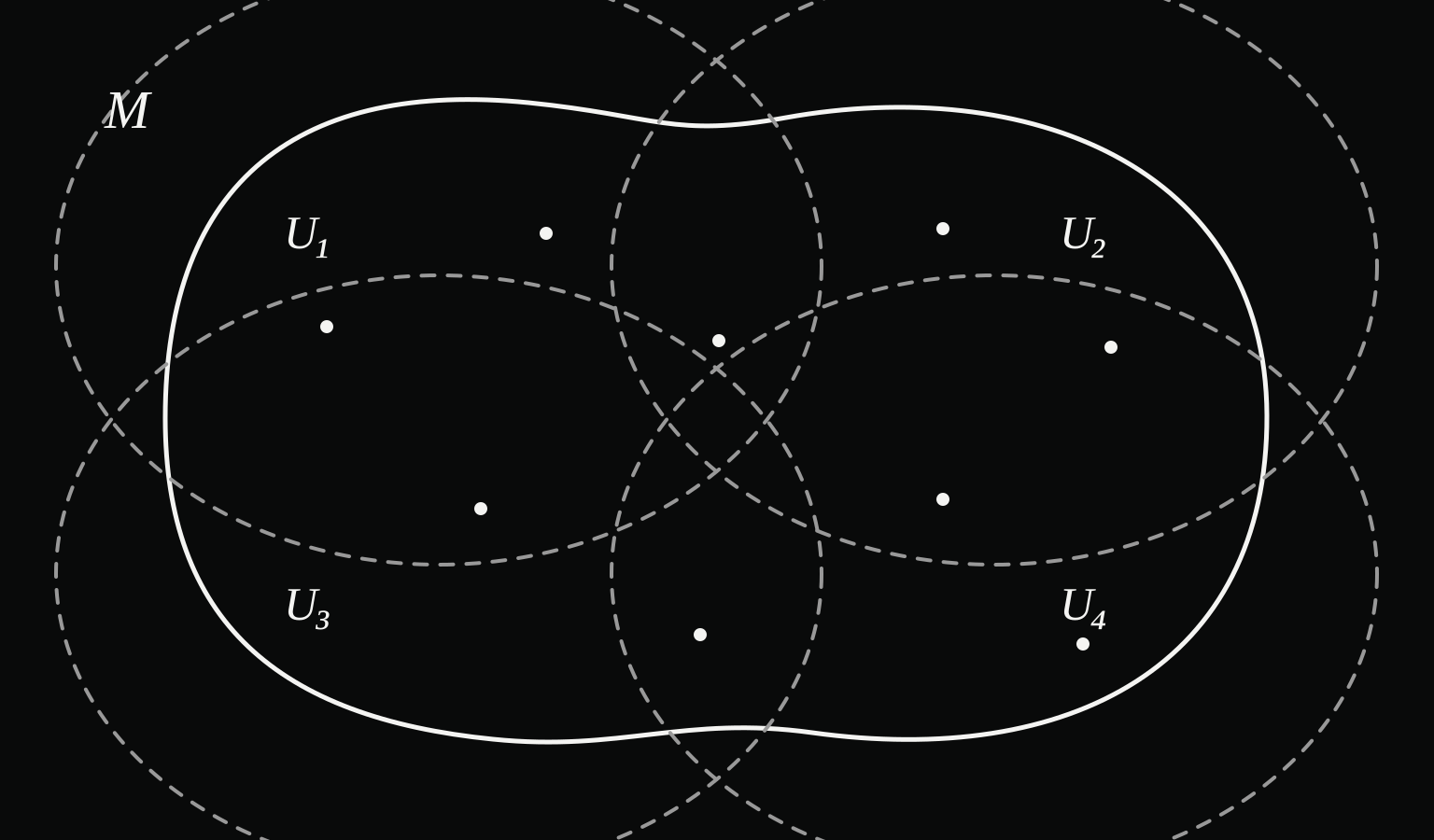
We may first look at compact metric spaces. Let M be a compact metric space, U an open cover of M.
The rough intuition is as follows.
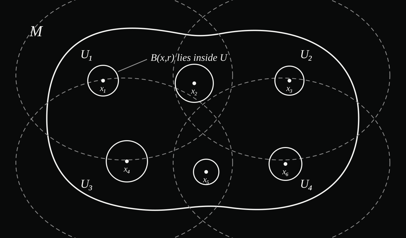
Each point is in some open set of the cover. Take a ball around each point, with radius small enough to still be wholly contained inside that open set (always possible, since open sets are exactly unions of such balls).
Now we have a ball around each point of M, each one wholly contained inside some member of the original cover.
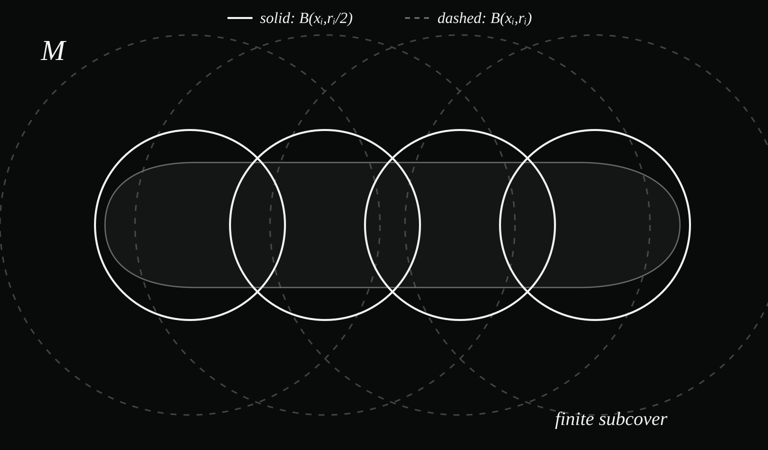
Halve each ball’s radius, keeping the same centre, so each half-radius ball sits wholly inside its own full-radius parent ball.
The half-radius balls still cover M (each point sits at the centre of its own), so take a finite subcover of these. Each ball in this finite subcover has a centre whose full-radius (unhalved) ball is still wholly contained inside some member of the original cover.
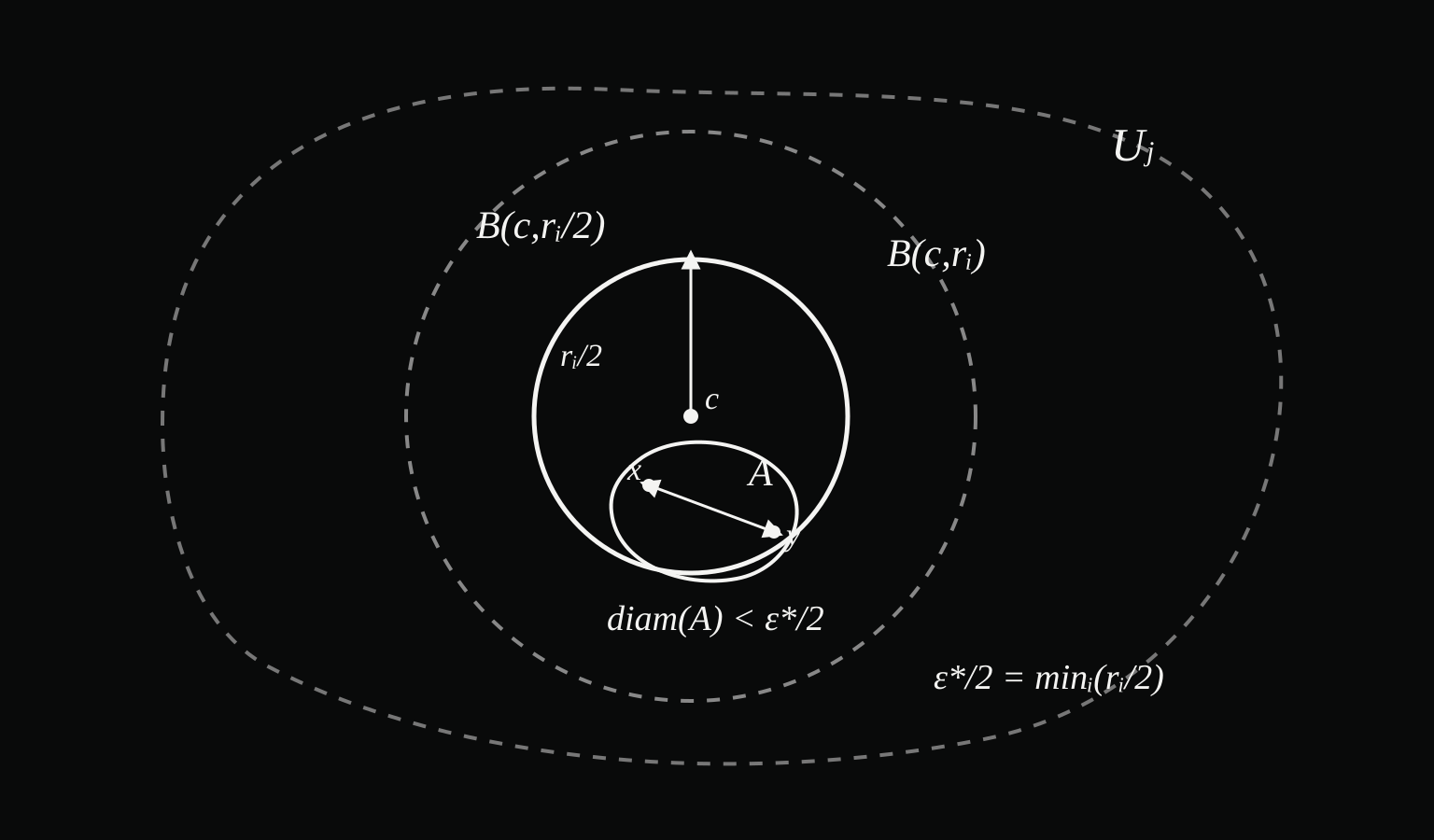
Now take the minimum of all these (finitely many) half-radii, call it ϵ∗/2. For any set of diameter less than ϵ∗/2, pick a point p in it, it lies inside one of the finitely many half-radius balls; every other point of the set is then within ϵ∗/2 of that p too, so within ϵ∗/2+ϵ∗/2=ϵ∗ of the centre at most, well within the full-radius parent ball, which sits inside a member of the original cover.
So any set of small enough diameter is contained in some member of the original cover.
The Lebesgue Number Theorem
Theorem. Let M be a compact metric space, and U be an open cover of M, there exists ϵ>0 such that whenever A⊂M and diam(A)<ϵ, then A⊂U for some U∈U. This ϵ of course depends on the cover itself.
Proof. for each m∈M take two balls (hehe) B(m,rm/2)⊂B(m,rm)⊂Um. Now take a finite subcover K of the half radius balls, then for each 1≤i≤∣K∣ we have B(mi,rmi/2)⊂B(mi,rmi)⊂Umi.
Now, let e=min1≤i≤∣K∣(rmi/2), this obviously exists since K is a finite set.
let A⊂M for which diam(A)<e, choose any point a∈A. since K covers M, we have some m for which a∈B(m,rm/2). for any point a′∈A, d(m,a′)≤d(m,a)+diam(A)<rm/2+e but e≤rm/2,
thus d(m,a′)<rm, therefore A⊂B(m,rm)⊂Um.
Lebesgue Numbers for Covering Maps
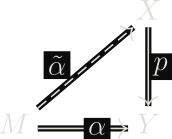
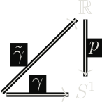
Now consider the setup from above, p:X→Y a covering map between topological spaces, and α:M→Y a continuous map to Y from a compact metric space M.
Theorem. There exists an e>0, such that any cover of M with open e-balls has the property that the image of a ball under α is contained inside an evenly covered set in Y.
Proof. for each y∈Y construct an open cover P by choosing an evenly covered neighborhood of y, Uy. the pre-images of these form an open cover V={α−1(Uy)∣Uy∈P} of M, since M is compact, let e+δ be the Lebesgue number for this cover.
then we know that for any ball B(m,e)⊂α−1(Uy) thus α(B(m,e))⊂Uy.
we shall call this e a (p,α) Lebesgue number.
That is to say, the thus obtained Lebesgue number quantifies the smallness of these evenly covered sets, relative to that metric space and that continuous map.
1 - Compact Metric Lifting
Small Covers of Compact Metric Spaces
We will first quickly show that a compact metric space is bounded. take some x∈M and construct open balls of increasing radius B(x,r),B(x,2r),… of course since the distance between any two points is finite, each point is contained inside some ball, now take the finite subcover of this cover, and notice that every point is contained inside the largest ball.
Next we shall show that for any e>0 a compact metric space can be covered with finitely many sets of diameter less than e.
consider any cover of this space with balls of radius e/4. take its finite subcover, the diameter of these balls is less than e/2, replace each ball with some e−δ diameter subset that contains the ball.
The Compact-Metric Lifting Theorem
We shall use this to solve the compact-metric lifting problem.
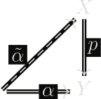
let M be a compact metric space, p:X→Y a covering map, α:M→Y a continuous map that needs to be lifted.
Theorem. The solution exists. Moreover, if for some m0∈M, we want α~(m0)=x0∈p−1(α(m0)), then the solution is unique.
Proof. let e be a (p,α) Lebesgue number. Then, M=⋃i=1NSi where diam(Si)<e. Moreover allow m0∈S1 (Si need not be closed or open or anything, but it should be connected).
Now, define Mt=⋃i=1tSi, αt=α∣Mt. we say that the lifting problem has a t-solution if there exists a unique α~t such that α~t(m0)=x0, and (of course) p∘α~t=αt.
We shall proceed inductively, solving instances using the relative lifting lemma. As usual, we show the inductive step first.
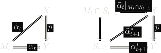
Suppose that this lifting problem has a t-solution. Denote α∣St+1 as αt+1∗, α~t∣Mt∩St+1 as βt, mainly for convenience.
Since each Si is connected, and Mt∩St+1 is a connected subset of St+1, and of course, α(Si)⊂U where U is evenly covered, the local lifting lemma says, there exists a unique α~t+1∗ for which, p∘α~t+1∗=αt+1∗ and α~t+1∗(M∩St+1)=βt(M∩St+1)=α~t(M∩St+1).
Pause here for a second, it is no coincidence that we choose the lift relative to the parts where Mt and St+1 overlap! we will glue these solutions together!!
This map is unique, since it is the piecewise join of the unique maps α~t and α~t+1∗. The two maps agree on Mt∩St+1, so the gluing lemma makes α~t+1 continuous. Finally, since m0∈Mt, we still have α~t+1(m0)=α~t(m0)=x0.
The base case is done by applying the local lifting lemma to S1, and doing it relative to {m0}, which is a single-element connected subset of S1.
2 - Lifting Paths and Homotopies
Path Lifting
Awesome! so now we can lift paths! can we lift loops? Not really, as p need not be injective.
Homotopy Lifting
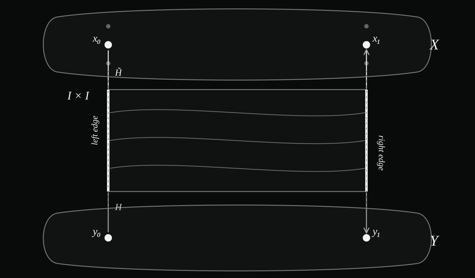
We can also lift homotopies! set M=[0,1]2 if the homotopy H:[0,1]2→Y fixes endpoints, that is, H(0,_)=c0 and H(1,_)=c1 (where c0,c1 are constant functions) meaning that at any homotopy slice H has the same two endpoints.
The left interval and right interval are of course connected, so their images under H~ must also be connected, but the preimage of y0 under p is a bunch of disconnected points, one on each sheet, thus, H~ is forced to pick one of those points.
i.e. H~ also fixes endpoints.
In particular, this means that though lifts of homotopy paths with fixed endpoints have fixed endpoints, the lift of a homotopy of loops, may not be a homotopy of loops but just a homotopy of paths.
3 - The Exponential Covering Map
Now, we go back to the map we’re dealing with.
where p(x)=ei2πx, we shall show p is a covering map.
for convenience, we will take the argument of a complex number to lie in [0,2π), where indeed, z=eia(z) where a(z) is this modified argument.
An open set in S1 can be given by an open interval I⊂[0,2π) as A={eit∣t∈I}. for each z∈S1 choose 1/2>e>0 such that Iz=(a(z)−e,a(z)+e)⊂[0,2π). we claim that Ez={eit∣t∈Iz} is evenly covered by p.
Notice,
p−1(Ez)=⨆k∈Z(2πa(z)−e+k,2πa(z)+e+k).
call such an interval Izk=(2πa(z)−e+k,2πa(z)+e+k). We choose e<1/2 as then the length of this interval is 2e/2π which is well smaller than 1.
we claim that for any k∈Z, p∗:=p∣Izk:Izk→Ez is a homeomorphism.
of course, p∗ is continuous, as it is a restriction of a continuous map. now, p∗(Izk)={ei2πx∣x∈Izk}.
Notice however that 2πx∈(a(z)−e+2πk,a(z)+e+2πk) but obviously, ei2πx=ei(2πx−2πk).
so p∗ is surjective. now, suppose p∗(x)=p∗(y), then ei2πx=ei2πy. without loss of generality y≥x, then we get y=x+h for some positive integer h. of course, since y,x∈Izk, y−x<1, thus y=x. Indeed p∗ is injective.
Define
qk:Ez⟶Izk,qk(v)=2πa(v)+k.
Here a:Ez→Iz is the continuous branch of the argument determined by
v=eia(v). We claim that qk=(p∗)−1.
Conversely, let x∈Izk. Then x−k∈Iz0, so
2π(x−k)∈Iz. Since a takes values in Iz, it follows that
a(p∗(x))=a(ei2πx)=2π(x−k).
Therefore
(qk∘p∗)(x)=2πa(p∗(x))+k=2π2π(x−k)+k=x.
Hence qk∘p∗=idIzk as well, proving that
qk=(p∗)−1.
Finally, qk is continuous because it is obtained from the continuous local
argument a∣Ez by scaling by 1/(2π) and translating by k.
Thus p∗:Izk→Ez is a homeomorphism. Since this holds for
every k∈Z, the set Ez is evenly covered by p.
Lifting Loops
To proceed, let us emphasize what the compact-metric lifting theorem says. it says, continuous maps from a compact metric space to a topological space can be lifted along a covering map to another topological space. In particular, it also says this lift is unique as long as its restriction on a connected subset of the metric space is determined.
choose k∈Z. Then, consider the set of loops on S1 with basepoint 1∈C, denoted by Ω(S1,1), and consider the set of paths P(R) on the reals. The compact-metric lifting theorem says that the map Lk:Ω(S1,1)→P(R) given by α↦α~k where α~k(0)=k is well defined, and is injective.
({0} is a connected subset of [0,1])
That is Lk takes a loop, and gives the unique lift of it, for which its image of zero is k.
at this point, I thought that any real number shift of a lift is another lift, I quickly realized that of course, this is not true, if you lift a loop, shift it only a tiny amount and project it back down, it is still morally the same loop but the basepoint has shifted, however, an integer shift will wrap back around to the same basepoint
Shifting Lifts
we claim that for any integer r, r⊕α~k:x↦r+α~k(x) is a lift of α.
in particular, (r⊕α~k)(0)=k+r, but α~k+r is the unique lift whose image of zero is k+r. Therefore, r⊕α~k=α~k+r whenever r is an integer.
The Endpoint Map
Another map we can define is ϕk:Ω(S1,1)→Z given by α↦α~k(1)−α~k(0). Well, why is the difference an integer? α is a loop, and α(1)=α(0)=1. thus, α~k(1),α~k(0)∈p−1(1)=Z.
Homotopy Invariance
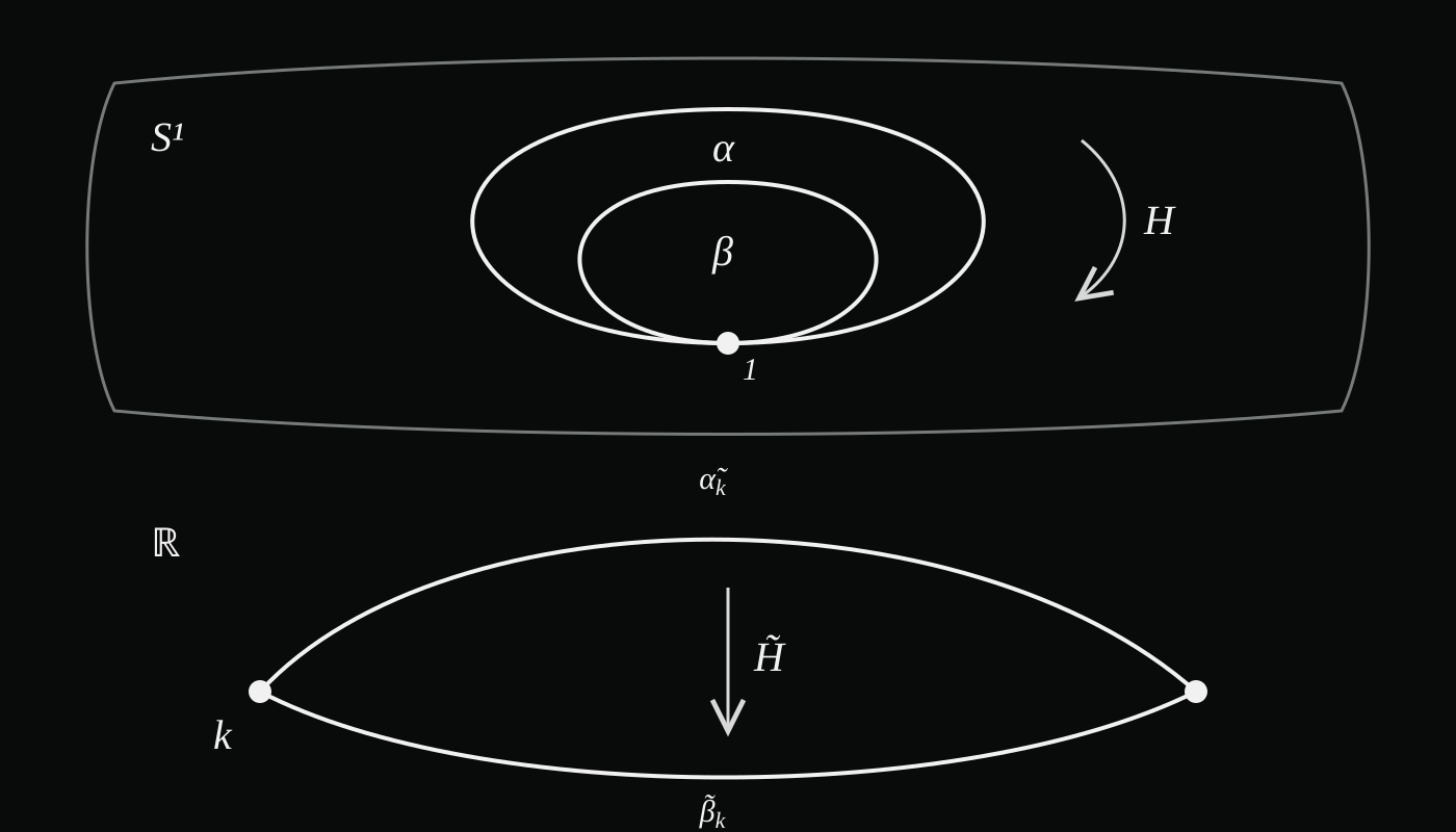
Now, we claim that whenever α∼β by homotopy of loops, then ϕk(α)=ϕk(β).
let H:[0,1]2→S1 be a homotopy from α to β.
of course, we can lift H, choose the unique lift H~ for which H~(0,0)=k.
of course, as shown earlier, if H fixes endpoints, then so does H~. That is to say, H~(0,_) and H~(1,_) are constant functions, moreover this means, H~(0,_)=k as a constant function.
obviously, H~(_,0),H~(_,1) are lifts of H(,0)=α,H(,1)=β respectively, moreover, they are the unique lifts whose image at 0 is k.
Indeed, H~(,0)=α~k,H~(,1)=β~k
well, of course then the endpoints of α~k,β~k are respectively equal, i.e. ϕk(α)=ϕk(β).
Thus, we can define without worry Φk:π1(S1,1)→Z by [α]↦ϕk(α).
Wow, this is a wild amount of setup!
The Fundamental Group of the Circle
Well, we may as well inspect Φ0, given by [α]↦α~0(1). We will show that it is a group homomorphism. i.e. Φ0([α∗β])=α~0(1)+β~0(1).
We can tell that we want to lift α∗β into some path p such that p(0)=0 and p(1)=α~0(1)+β~0(1).
Naively, one might think of joining α~0 with β~0, but their only common point might be 0 itself, in particular, it may be that α~0(1)=0=β~0(0). But what we do know, is that α~0(1)=q∈Z!
As seen earlier, β~q=q⊕β~0.
we claim that the lift with startpoint 0 of the product is
composing the above map with the covering map p piecewise, it is not hard to see that it lifts α∗β. of course, the map agrees at the common point, (notice q=α~0(1)). and (L0(α∗β))(0)=0. (as defined)
Now notice that L0(α∗β)(1)=β~q(1)=q+β~0(1)=α~0(1)+β~0(1)=Φ0([α∗β]).
i.e. Φ0 is a homomorphism of groups!
we shall next show that Φ0 is injective. suppose Φ0([α])=Φ0([β]) then of course α~0(1)=β~0(1), i.e. α~0,β~0 have the same endpoints. (at this point, we think these two paths are homotopic, and we can project it down via p to show α is homotopic to β)
Define U:[0,1]2→R given by U(t,s)=(1−s)α~0(t)+sβ~0(t). Indeed, U is a homotopy (with endpoints fixed) from α~0 to β~0. (The reader is asked to pause and verify.)
so, p∘U:[0,1]2→S1 is indeed a continuous map. Since both endpoints, namely 0, α~0(1)=β~0(1)∈Z,
p∘U(0,_)=p(0)=1 and p∘U(1,_)=p(α~0(1))=1, we have each slice p∘U(_,s) is a loop in S1.
of course, p∘U(,0)=p∘α~0=α and similarly, p∘U(,1)=β
thus p∘U is a homotopy of loops, from α to β, i.e. [α]=[β].
A nice thing about showing Φ0 is a homomorphism, is that it is enough to show a loop α for which Φ0([α])=1∈Z to show surjectivity.
consider the loop p∣[0,1]:[0,1]→S1 it is clear that the inclusion map ι:[0,1]→R lifts this loop, (by definition, p∣[0,1]=p∘ι).
and of course Φ0([p∣[0,1]])=ι(1)=1.
It directly follows that Φ0([(p∣[0,1])−1])=−1. And thus, any integer is formed by taking Φ0 on repeated products.
Thus finally Φ0:π1(S1,1)→Z is a bijective homomorphism. i.e.
π1(S1,1)≅Z
LET’S GO!!
4 - Homotopy Equivalence and Fundamental Groups
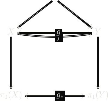
Recall that two topological spaces X,Y (with base points) are homotopy equivalent if there exists a pair of continuous basepoint preserving maps f:X→Y,g:Y→X such that g∘f is homotopic to idX and f∘g is homotopic to idY.
if the fundamental group functor π1:Top∗→Grp is really about homotopy, then homotopy equivalent spaces should have isomorphic fundamental groups.
The above diagram isn’t exactly a commutative diagram in some fixed category, but it uses the fact that π1 takes continuous maps to a new map, that sends a homotopy class of loops to the class induced by composing a representative with the map.
i.e. π1(f):[α]↦[f∘α].
due to functoriality, π1(g)∘π1(f)=π1(g∘f):[α]↦[g∘f∘α].
let H:X×[0,1]→X be a homotopy from g∘f to idX.
H∘(α×id[0,1]):[0,1]2→X is a homotopy from g∘f∘α to α,
i.e. g∘f∘α∼α.
similarly if β is a loop on Y, then f∘g∘β∼β.
i.e. π1(g),π1(f) are inverses of each other.
i.e. π1(X)≅π1(Y).
The Punctured Plane and the Circle
Now, finally we will show that C−{0}=C∗ is homotopy equivalent to S1.
set f:C∗→S1 defined by z↦z/∣z∣ and ι:S1→C∗ the inclusion map.
of course, f∘ι=idS1 as is, now, consider ι∘f:C∗→C∗.
we want to construct a homotopy H:C∗×[0,1]→C∗ that is continuous, and takes idC∗ to ι∘f.
as usual we will fade one function out, and fade the other one in.
H(z,t)=(1−t)z+∣z∣tz=((1−t)+∣z∣t)z
Notice carefully that we are quite illiterate in analysis, so we will prove the continuity of the maps involved in a later note (it should be pretty chill, however this note is already getting too long).
But it does seem like continuous functions into the complex numbers can be added, composed and multiplied and if you removed the zero, can also be inverted. This is an interesting aside,
5 - Continuous Maps into Topological Fields
Enter Topological Fields.
A topological space (X,+,⋅) is a topological field, if it’s a field such that the following maps are continuous.
+,⋅:X2→X (product topology on X2) and (_)−1:X∗→X∗ (X without zero).
Let X be a topological field and Y a topological space. Let
C(Y,X)={f:Y→X∣f is continuous}.
Define the operations pointwise.
(f+g)(y)=f(y)+g(y),(fg)(y)=f(y)g(y).
And if f(y)=0 for every y, define
f−1(y)=f(y)−1.
Now we just need to check that these things are actually continuous.
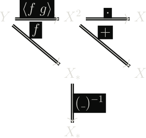
If f,g∈C(Y,X), then
(f,g):Y→X2,y↦(f(y),g(y))
is continuous, since f and g are continuous and X2 has the product topology.
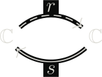
Warning. The above diagram is NOT A COMMUTATIVE DIAGRAM, I have deliberately drawn it that way, it is just to illustrate the compositions on each path.
Indeed, if you follow each path pointwise, you get fg:Y→X, f+g:Y→X, f−1:Y→X∗, which are compositions of continuous maps.
That is to say, continuous maps into topological fields are closed with respect to algebraic operations, (the inverse is the pesky one as usual).
Note that we are not saying that these maps themselves form a field (they form a ring of course).
Now we need to show that C is a topological field, we will do so in a later note.
6 - No Continuous Square Root
Now, back to the main thread.
The machinery we have built so far is powerful, and will be used over and over. Let us do a demonstration.
We claim that there is no continuous square-root function on C. Write
s:C⟶C,s(z)=z2.
A continuous square root would be a map r:C→C such that
s∘r=idC; that is, r would be a section of
the squaring map.
if an r existed on the non-zero complex numbers, we could bring it back to
all of C by filling in r(0)=0.
indeed, take any open ball B(0,e) around the origin in the codomain. since
r(z)2=z, we have
r−1(B(0,e))=B(0,e2).
the right hand side is an open ball around the origin in the domain. Thus the
extension is continuous at 0, and it was already continuous everywhere else.
Therefore, it is enough to show that there is no continuous square root on
C∗=C∖{0}.
Assume for contradiction that r:C∗→C∗ exists.
Since r(1)=±1, replacing r by the continuous square root
(−r)(z)=−r(z) if necessary lets us assume r(1)=1. Thus r and s are
based maps at 1, and s∘r=idC∗.
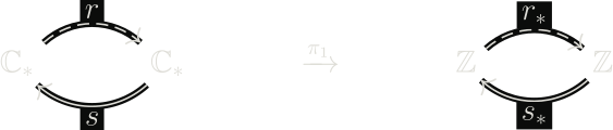
Applying π1 gives
π1(s)∘π1(r)=π1(s∘r)=idπ1(C∗,1).
The Fundamental Group Obstruction
We claim that the map induced by squaring is the doubling map.
π1(s)=d:Z⟶Z,d(n)=2n.
Assuming this claim, call h=π1(r). The equation above becomes
d∘h=idZ.
But no such h can exist. plugging in 1 would give 2h(1)=1, which is
impossible since h(1) is an integer.
Squaring Induces Doubling
Proof of the claim. first, let us be clear about what the element
1∈Z represents. Recall that
Φ0:π1(S1,1)⟶Z
sends the class of the loop
γ=p∣[0,1],γ(t)=ei2πt,
to 1, since its lift starting at 0 is t↦t and ends at 1.
Now let ι:S1↪C∗ be the inclusion. We have
already shown that
ι∗:π1(S1,1)⟶π1(C∗,1)
is an isomorphism. Thus, when we identify π1(C∗,1) with
Z using Φ0∘ι∗−1, we get
(Φ0∘ι∗−1)(ι∗([γ]))=Φ0([γ])=1.
So the same loop, now regarded as a loop in C∗, represents the
element 1 there as well.
well, π1(s):Z→Z is a group homomorphism, and a group
homomorphism out of Z is completely determined by where it sends
1.
then
(s∘γ)(t)=γ(t)2=ei4πt.
the lift of this loop which starts at 0 is just t↦2t, and it ends
at 2. Thus π1(s) sends 1 to 2.
but now the entire homomorphism is forced. for every n∈Z,