Algebra - 3

In this entry, we will resolve at least one promise from the last entry.

1 - Cones as Comma Categories

Last time, we saw that given an index category $\mathsf{J}$, the category of diagrams in $\mathsf{C}$ of shape $\mathsf{J}$ is just the functor category $\operatorname{Diag}(\mathsf{J}, \mathsf{C})$.

We took an interest in special diagrams that very much resemble objects of $\mathsf{C}$ itself, called constant diagrams $\underline{A}$, which take every object of $\mathsf{J}$ to the object $A \in \mathsf{C}$, and every morphism of $\mathsf{J}$ to the identity on $A$.

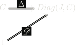
In particular, we saw the diagonal functor $\Delta: \mathsf{C} \to \operatorname{Diag}(\mathsf{J}, \mathsf{C})$, which takes each object $A$ to the constant diagram $\underline{A}$, and each morphism $f: A \to B$ to the natural transformation $\underline{A} \Rightarrow \underline{B}$ whose every component is $f$.

Moreover, we saw that a fixed diagram $D \in \operatorname{Diag}(\mathsf{J},\mathsf{C})$ can equivalently be represented as a functor $\mathscr{D}: \mathsf{1} \to \operatorname{Diag}(\mathsf{J},\mathsf{C})$, where the lone object $*$ of $\mathsf{1}$ is sent to $D$.

Thus, we saw that the category of cones over $D$ in $\mathsf{C}$ is the comma category of the two functors $\Delta, \mathscr{D}$.

The comma category $(\Delta \downarrow \mathscr{D})$ has objects $(A, *, u: \Delta(A) \to \mathscr{D}(*))$, that is, pairs $(A, u: \underline{A} \Rightarrow D)$, exactly a cone over $D$ with apex $A$. We may as well take objects of this category as the definition of a cone, but it’s nice to check that it embodies the naive definition of a cone.

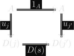
Notice that $u$ is a natural transformation between two functors $\underline{A}, D$, both from $\mathsf{J}$ to $\mathsf{C}$. But notice that for any $j \in \mathsf{J}$, $\underline{A}(j) = A$, and for any morphism $s: j \to j'$ in $\mathsf{J}$, $\underline{A}(s) = 1_A$. In particular, every component of $u$, call it $u_j$, is a morphism $A \to D(j)$.

Now consider a morphism $s: j \to j'$ in $\mathsf{J}$. The naturality square looks like:

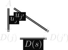
Since the top arrow is $1_A$, this simplifies to the triangle:

with commutativity condition $D(s) \circ u_j = u_{j'},$ for every morphism $s: j \to j'$ in $\mathsf{J}$. This is exactly the naive, componentwise definition of a cone: a collection of morphisms $u_j: A \to D(j)$, one for each object of $\mathsf{J}$, compatible with every morphism of the diagram.

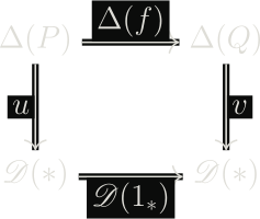
What are morphisms here? Of course, as with any comma category, a morphism in $(\Delta \downarrow \mathscr{D})$ from $(P,u)$ to $(Q,v)$ is a pair of morphisms $(f: P\to Q,\ 1_*: *\to *)$, one in $\mathsf{C}$, one in $\mathsf{1}$. Since $\mathsf{1}$ has only the identity morphism, this is really just identified with a morphism $f: P \to Q$ in $\mathsf{C}$.

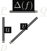
Of course, it’s not just any morphism, but one making the following square commute:

Since $\mathscr{D}(1_*) = 1_D$, this collapses to $v \circ \Delta(f) = u,$ an equation of natural transformations $\underline{P} \Rightarrow D$. That is, $f: P \to Q$ is a morphism of cones exactly when postcomposing $Q$‘s cone with $\Delta(f)$ recovers $P$‘s cone.

In particular, $\Delta(f)$ is the natural transformation from the constant diagram at $P$ to the constant diagram at $Q$, all of whose components are $f$. We can use componentwise reasoning here, but at the end of the day, objects in the target category $\operatorname{Diag}(\mathsf{J},\mathsf{C})$ are all functors, and morphisms are natural transformations, and the equation above is an equation of natural transformation composition.

That is to say, we have the following commutative (as an evaluation of the one above) diagram, whose objects are functors and whose morphisms are natural transformations:

Notice that each $\underline{P}, \underline{Q}, D$ are functors from $\mathsf{J}$ to $\mathsf{C}$. Thus, we just want the components $v_{\Delta(f)_{(j)}} \circ u_j$ wait, let’s restate this properly: we want, for each $j \in \mathsf{J}$, $v_j \circ \Delta(f)_j = u_j.$ Notice that for any object $j$, $\Delta(f)_j$ simply sends the object $\underline{P}(j) = P$ to the object $\underline{Q}(j) = Q$ via $f$, that is, $\Delta(f)_j = f$ for every $j$. So every component of $u$ is a morphism from $P$ to $D(j)$ in $\mathsf{C}$, and every component of $v$ is a morphism from $Q$ to $D(j)$ in $\mathsf{C}$, call them $u_j, v_j$ respectively. We want the triangle to commute, that is, $v_j \circ f = u_j \quad \text{for each } j.$

---

2 - Whiskering

Composing natural transformations can be extended beyond parallel functors.

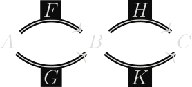
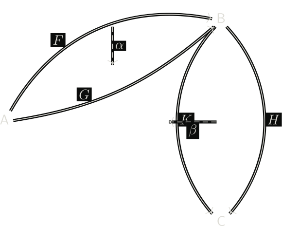
Imagine categories $\mathsf{A}, \mathsf{B}, \mathsf{C}$, functors $F, G: \mathsf{A}\to\mathsf{B}$, and functors $H, K: \mathsf{B}\to\mathsf{C}$. Let $\alpha: F\Rightarrow G$ be a natural transformation, and $\beta: H\Rightarrow K$ be a natural transformation.

with $\alpha: F\Rightarrow G$ drawn between the two arrows $\mathsf{A}\to\mathsf{B}$, and $\beta: H\Rightarrow K$ drawn between the two arrows $\mathsf{B}\to\mathsf{C}$.

Let’s first tackle the simplest piece we actually need: post-composing a single functor with a natural transformation. Suppose we forget $\beta$ for a moment, and just have $\alpha: F \Rightarrow G$ (both $\mathsf{A}\to\mathsf{B}$), and a single functor $H: \mathsf{B}\to\mathsf{C}$. We want to build a natural transformation $HF \Rightarrow HG$, using $\alpha$ and $H$ alone.

For each object $X \in \mathsf{A}$, $\alpha$ gives us a morphism $\alpha_X: F(X) \to G(X)$ in $\mathsf{B}$. Since $H$ is a functor, we can apply it: $H(\alpha_X): HF(X) \to HG(X)$, a morphism in $\mathsf{C}$. Define $(H\alpha)_X := H(\alpha_X).$

Check naturality. For $s: X\to Y$ in $\mathsf{A}$, we need $(H\alpha)_Y \circ HF(s) = HG(s) \circ (H\alpha)_X$, i.e. $H(\alpha_Y)\circ H(F(s)) = H(G(s))\circ H(\alpha_X)$. Since $H$ is a functor, this is $H(\alpha_Y \circ F(s)) = H(G(s)\circ \alpha_X)$, and this follows by applying $H$ to both sides of $\alpha$‘s own naturality square, $\alpha_Y\circ F(s) = G(s)\circ\alpha_X$, which holds since $\alpha$ is natural.

So $H\alpha: HF \Rightarrow HG$ is a genuine natural transformation, built purely from $\alpha$ and $H$. This operation, sticking a functor onto one side of a natural transformation, is called whiskering.

On the other hand, one wonders the following setup: $F$ a functor from $\mathsf{A}$ to $\mathsf{B}$, and $H,K$ functors from $\mathsf{B}$ to $\mathsf{C}$, with a natural transformation $\beta: H\Rightarrow K$ between them. We want a natural transformation between $HF$ and $KF$.

Of course, our gut tells us that we must define the component $(\beta F)_X$ to simply be $\beta_{F(X)}$, that is, pre-composing $F$ with a natural transformation has components given by $\beta$, evaluated after first applying the functor $F$: $(\beta F)_X := \beta_{F(X)}.$

Check naturality. For $s: X\to Y$ in $\mathsf{A}$, we need $(\beta F)_Y \circ HF(s) = KF(s)\circ(\beta F)_X$, i.e. $\beta_{F(Y)} \circ H(F(s)) = K(F(s))\circ \beta_{F(X)}.$ But this is exactly $\beta$‘s own naturality square, applied at the morphism $F(s): F(X)\to F(Y)$ in $\mathsf{B}$, which holds since $\beta$ is natural.

So $\beta F: HF \Rightarrow KF$ is the needed natural transformation.

Now to compose $\alpha$ with $\beta$:

The question becomes: how can we make a natural transformation between the functors $HF$ and $KG$? And if our whiskering and usual vertical composition are worthy of the title “composite,” it had better be that if we have multiple “composites” of $\alpha$ and $\beta$, they turn out to be equal.

The first way is: whisker $F$ before $\beta: H \Rightarrow K$ to get $\beta F: HF \Rightarrow KF$. Now whisker $K$ after $\alpha: F \Rightarrow G$ to get $K\alpha: KF \Rightarrow KG$. Notice that both these transformations are between functors from $\mathsf{A}$ to $\mathsf{C}$, i.e. we can compose them as usual, giving us a candidate $K\alpha \circ \beta F$.

Another way is: whisker $H$ after $\alpha: F \Rightarrow G$ to get $H\alpha: HF \Rightarrow HG$. Now whisker $G$ before $\beta: H \Rightarrow K$ to get $\beta G: HG \Rightarrow KG$, giving us another candidate $\beta G \circ H\alpha$.

We know that both these candidates are of course valid natural transformations, however, they had better be equal, that is, have all the same components.

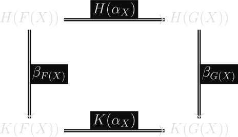
Consider an object $X$ in $\mathsf{A}$. Indeed, $\alpha_X: F(X) \to G(X)$ in $\mathsf{B}$. Thus, $H(\alpha_X): H(F(X)) \to H(G(X))$ is a morphism in $\mathsf{C}$. Similarly, $\beta_{G(X)}: H(G(X)) \to K(G(X))$; the vertical composite of those two simply composes both components.

On the other hand, we have $\beta_{F(X)}: H(F(X)) \to K(F(X))$, a morphism in $\mathsf{C}$, and similarly $K(\alpha_X): K(F(X)) \to K(G(X))$.

Staring at the above diagram, it is not hard to see that it’s just the naturality square for $\beta$, applied at the morphism $\alpha_X: F(X) \to G(X)$. Thus, the two paths are equal.

---

3 - Free Groups

We shall seemingly cut to something else, but don’t worry, we will bring it back.

Suppose you have a set $S$. One might think about defining the set of all finite-length words in $S$, this depicting some sort of monoid-type structure, with the empty word serving as an identity.

It’s not entirely clear how the binary operator is recovered here, and what the rules should be. So let’s build it up.

Notice, the empty set has the capacity only to make the empty word, so we know that the free group on the empty set should just be, up to isomorphism, the trivial group with just an identity.

What about a singleton? Well, you have $S = \{a\}$. You will have to include the empty word, and a symbol that is the inverse of $a$, call it $a^{-1}$. It is not difficult to see that in this case, $FG(S)$ consists of words $a^m$ or $(a^{-1})^m$ for some $m \in \mathbb{N}$ (do an induction argument, or otherwise notice that $aa^{-1}$ or $a^{-1}a$, as subwords, evaluate to the empty word).

In particular, defining $a^{-z} := (a^{-1})^z$ and $a^0$ to be the empty word, it is easy to see that this group is isomorphic to $(\mathbb{Z}, +)$.

---

4 - The Fundamental Group of Topological Spaces

Let $(X, x^*)$ be a topological space with a chosen basepoint. One way to study a topological space is to look at the algebra of loops (up to continuous deformation) on that space.

Indeed, a loop is a continuous map $l: [0,1] \to X$ with $l(0) = l(1) = x^*$. At this point, the reader can stop and check out my topology note.

Of course, we want to consider homotopy classes of such maps. We need a product on $\operatorname{Hom}([0,1],X)/\sim$, where $\sim$ is the homotopy relation.

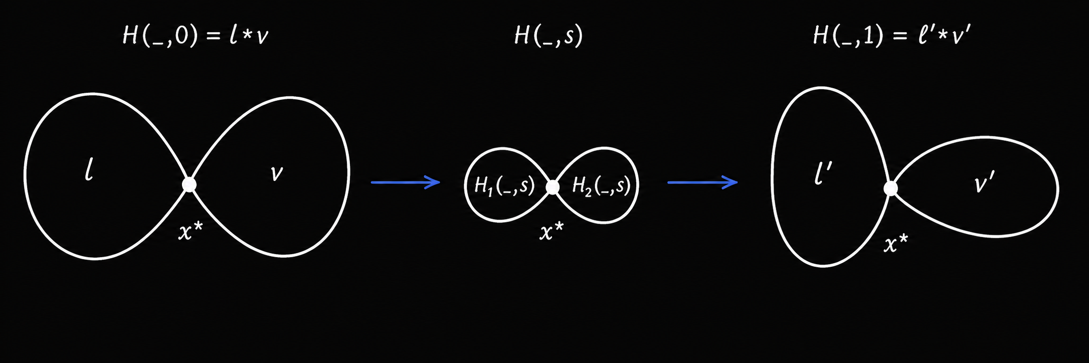
Well, let $[l], [v]$ be two homotopy classes. By choosing representatives $l, v$, we may construct $l *_{1/2} v: [0,1] \to X$, defined by

$$t \mapsto \begin{cases} l(2t) & t \in [0, 1/2] \\ v(2t-1) & t \in [1/2, 1] \end{cases}$$

Again, we invoke the gluing lemma from the topology note to show that $l*v$ is a continuous map. But of course, we want the induced class $[l*v]$ to be well-defined, that is to say, if $l \sim l'$ and $v \sim v'$, we want $l*v \sim l'*v'$.

Let $H_1, H_2: [0,1]^2 \to X$ be the homotopies between $l, l'$ and $v, v'$ respectively. That is, $H_1, H_2$ are continuous maps (product topology on $[0,1]^2$) with $H_1(\_,0) = l$, $H_1(\_,1) = l'$, and $H_2(\_,0) = v$, $H_2(\_,1) = v'$.

Notice that these loops are basepoint preserving, that is, every homotopy slice $H_1(\_,s)$ and $H_2(\_,s)$ must be a continuous map $[0,1] \to X$ such that $0, 1$ both go to the basepoint $x^*$.

This suggests we should glue $H_1$ and $H_2$ at $t=1/2$, at double speed, for every fixed value of $s$, exactly as we did for $l*v$ itself. Define $H: [0,1]^2 \to X$ by

$$H(t,s) = \begin{cases} H_1(2t,\,s) & t \in [0, 1/2] \\ H_2(2t-1,\,s) & t \in [1/2, 1] \end{cases}$$

At the seam $t=1/2$, the two branches must agree for every $s$: the top branch gives $H_1(1,s)$, the bottom gives $H_2(0,s)$. Since $H_1, H_2$ are basepoint-preserving homotopies, $H_1(1,s) = x^* = H_2(0,s)$ for every $s \in [0,1]$, so the two definitions agree along the entire seam, not merely at $s=0,1$.

By the gluing lemma, $H$ is therefore continuous. Checking the endpoints in $s$:

$$H(t,0) = \begin{cases} H_1(2t,0) = l(2t) & t\in[0,1/2] \\ H_2(2t-1,0) = v(2t-1) & t\in[1/2,1] \end{cases} = (l*v)(t),$$ $$H(t,1) = \begin{cases} H_1(2t,1) = l'(2t) & t\in[0,1/2] \\ H_2(2t-1,1) = v'(2t-1) & t\in[1/2,1] \end{cases} = (l'*v')(t).$$

So $H$ is a homotopy from $l*v$ to $l'*v'$, and moreover $H$ is itself basepoint preserving (each slice $H(\_,s)$ sends $0$ and $1$ to $x^*$, since $H_1(0,s)=x^*=H_2(1,s)$ for every $s$). Thus $l*v \sim l'*v'$, and the product $[l]*[v] := [l*v]$ is well defined on homotopy classes.

Now, to show that this product is associative, it is sufficient to show that $*$ on representatives is associative up to homotopy. That is, to show that $(l*v)*u \sim l*(v*u)$.

Associativity

Let’s just do the interval math over here.

$(l*v)*u$ expands (unwinding the outer product, then the inner one) to

$$((l*v)*u)(t) = \begin{cases} l(4t) & t\in[0,1/4] \\ v(4t-1) & t\in[1/4,1/2] \\ u(2t-1) & t\in[1/2,1] \end{cases}$$

and similarly, $l*(v*u)$ expands to

$$(l*(v*u))(t) = \begin{cases} l(2t) & t\in[0,1/2] \\ v(4t-2) & t\in[1/2,3/4] \\ u(4t-3) & t\in[3/4,1] \end{cases}$$

Notice the two are literally the same three pieces, $l$ then $v$ then $u$, just with the breakpoints sitting in different places, $1/4,1/2$ versus $1/2,3/4$.

Let $p_1(s) = \frac{1+s}{4}$, $p_2(s) = \frac{2+s}{4}$, so $p_1(0),p_2(0) = 1/4,1/2$ and $p_1(1),p_2(1) = 1/2,3/4$.

Define the reparametrization maps of the three pieces,

$$\rho_1(t,s) = \frac{t}{p_1(s)}, \qquad \rho_2(t,s) = \frac{t-p_1(s)}{p_2(s)-p_1(s)}, \qquad \rho_3(t,s) = \frac{t-p_2(s)}{1-p_2(s)},$$

each continuous.

Now define $H$ by

$$H(t,s) = \begin{cases} l(\rho_1(t,s)) & t \in [0,\,p_1(s)] \\ v(\rho_2(t,s)) & t \in [p_1(s),\,p_2(s)] \\ u(\rho_3(t,s)) & t \in [p_2(s),\,1] \end{cases}$$

Each piece is a composite of two continuous functions, $l\circ\rho_1$, $v\circ\rho_2$, $u\circ\rho_3$, hence continuous.

At the seams, $t=p_1(s)$ gives $l(1)=x^*$ on one side and $v(0)=x^*$ on the other, for every $s$, and same story at $t=p_2(s)$ with $v(1)=x^*=u(0)$. So we may invoke the gluing lemma, and $H$ is continuous on all of $[0,1]^2$.

Plugging in $s=0,1$ recovers $(l*v)*u$ and $l*(v*u)$ exactly, and $H(0,s)=l(0)=x^*$, $H(1,s)=u(1)=x^*$ for every $s$, so $H$ stays a based loop throughout.

Thus $(l*v)*u \sim l*(v*u)$, and $*$ is associative on homotopy classes.

Inverses

Now the inverse. It should just be reversing the interval.

Given a loop $l$, define $\bar l(t) := l(1-t)$, clearly continuous, and $\bar l(0)=x^*=\bar l(1)$. We want $l*\bar l \sim e_{x^*}$.

$(l*\bar l)(t) = \begin{cases} l(2t) & t\in[0,1/2] \\ \bar l(2t-1) & t\in[1/2,1] \end{cases} = \begin{cases} l(2t) & t\in[0,1/2] \\ l(2-2t) & t\in[1/2,1] \end{cases}$

so it walks out along $l$ then walks straight back.

Define $H(t,s) = \begin{cases} l((1-s)2t) & t\in[0,1/2] \\ l((1-s)(2-2t)) & t\in[1/2,1] \end{cases}$

at $s=0$ this is just $l*\bar l$, at $s=1$ both pieces are $l(0)=x^*$, so $H(\cdot,1) = e_{x^*}$.

Each piece is $l$ composed with a continuous reparametrization, hence continuous. At the seam $t=1/2$, both pieces give $l(1-s)$, matching for every $s$, so we may invoke the gluing lemma and $H$ is continuous.

$H(0,s)=l(0)=x^*$, $H(1,s)=l(0)=x^*$ for every $s$.

Thus $l*\bar l \sim e_{x^*}$, and symmetrically $\bar l * l \sim e_{x^*}$, so $[\bar l]$ is the two-sided inverse to $[l]$.

The group thus obtained is called the fundamental group of $X$ (at basepoint $x^*$). Now I must mention that changing basepoints gives isomorphic fundamental groups so long as the space $X$ is path connected.

Definition of the Fundamental Group

Let $(X,x^*)$ be a topological space with basepoint $x^*$. The fundamental group of $X$ at $x^*$, denoted $\pi_1(X,x^*)$, is the set of homotopy classes of loops based at $x^*$,

$$\pi_1(X,x^*) := \{ l : [0,1]\to X \mid l \text{ continuous}, \ l(0)=l(1)=x^* \} \big/ \sim,$$

equipped with the product $[l][v] := [l*v]$.

This is a group: $*$ is well defined on classes, associative up to homotopy (hence associative on classes), the class of the constant loop $e_{x^*}$ is a two-sided identity, and $[\bar l]$, the class of the reversed loop, is a two-sided inverse to $[l]$.

---

5 - Functoriality of the Fundamental Group

Now, consider the category of groups $\mathsf{Grp}$ and the category of pointed topological spaces $\mathsf{Top}^*$. We claim that $\pi_1$, as defined above, with the right choice of “image of continuous maps,” is a functor from $\mathsf{Top}^*$ to $\mathsf{Grp}$.

Suppose $f: (X,x^*) \to (Y,y^*)$ is a continuous basepoint-preserving map. Then, of course, $\pi_1(X,x^*)$ contains homotopy classes of loops $l: [0,1] \to X$, and we may as well send $[l] \mapsto [f\circ l]$ via $\pi_1(f)$.

For any representative $l$ of $[l]$, it’s easy to show that $f\circ l: [0,1] \to Y$ is a loop on $Y$. Of course, the composed map is continuous, and given that $l(0)=l(1)=x^*$, we get $f(l(0)) = f(l(1)) = y^*$.

Now we need to show that the map between equivalence classes is well defined, as we have done so many times now. That is, whenever $l \sim l'$, where $l,l'$ are loops on $X$, we want to show that $f\circ l \sim f\circ l'$.

Let $H: [0,1]^2 \to X$ be a homotopy from $l$ to $l'$. We claim that $f\circ H: [0,1]^2 \to Y$ is a homotopy from $f\circ l$ to $f\circ l'$.

Firstly, it’s clear that $f\circ H$ is continuous. Next, we claim that any slice $f\circ H(\_,s)$ is a loop on $Y$: since $H(\_,s)$ is a loop, $H(0,s)=H(1,s)=x^*$ for each $s\in[0,1]$, so, composing with $f$, $f\circ H(\_,s)$ is indeed a loop.

Next, since $H(\_,0)=l$ and $H(\_,1)=l'$, we get $f\circ H(\_,0) = f\circ l$ and $f\circ H(\_,1) = f\circ l'$.

$\pi_1(f)$ Is a Homomorphism

Consider $\pi_1(f)([l][v])$. By definition of our product on equivalence classes, this is equal to $\pi_1(f)([l*v]) = [f\circ(l*v)]$.

On the other hand, $\pi_1(f)([l])\,\pi_1(f)([v]) = [f\circ l][f\circ v] = [(f\circ l)*(f\circ v)]$, the last equality again by definition of our product.

Now, the reader can convince themselves that, picking representatives $l,v$, the functions $(f\circ l)*(f\circ v)$ and $f\circ(l*v)$ are literally equal, so the two equivalence classes are equal too.

Now it’s clear that $\pi_1$ preserves identity maps. Thus only one question remains: is $\pi_1(g\circ f) = \pi_1(g) \circ \pi_1(f)$? Well, $\pi_1(g\circ f)$ sends a loop $[l]$ to $[g\circ f \circ l]$, which is indeed $\pi_1(g)([f \circ l]) = \pi_1(g)(\pi_1(f)([l]))$.

---

6 - Towards the Fundamental Group of the Torus

Let us compute some homotopy groups (in general this is a pain).

Consider the torus. It is built by identifying the ends of a cylinder as equivalent (with the same direction). A cylinder itself is built by identifying the top and bottom of a square as equivalent.

Consider the space $S = [0,1]^2$ with the standard topology (inherited as a subspace). We say

$$(x,y) \sim (x',y') \iff (x,y)=(x',y') \ \text{ or } \ \big(y=y' \text{ and } \{x,x'\}=\{0,1\}\big) \\$$ $$\text{ or } \ \big(x=x' \text{ and } \{y,y'\}=\{0,1\}\big).$$

To get the torus, put the quotient topology on $S/\sim$, i.e., $U$ is open if and only if $\pi^{-1}(U)$ is open in $S$, where $\pi: S \to S/\sim$ is the canonical projection map.

First, we shall show that $S/\sim$ is path connected. Note that a topological space $X$ is path connected if for any $x,y \in X$, there exists a continuous map $c_{x,y}: [0,1] \to X$ such that $c_{x,y}(0) = x$, $c_{x,y}(1) = y$.

Let $[x],[y] \in S/\sim$. Pick representatives $x' \in [x]$, $y' \in [y]$.

Notice that the map $u: [0,1] \to S$ given by $u(t) = x' + t(y'-x')$ is continuous, where of course $x',y' \in [0,1]^2$ and the algebra is that of vector spaces. Also, $u(0) = x'$, $u(1) = y'$.

Obviously then, $\pi \circ u$ is continuous, and $\pi\circ u(0) = \pi(x') = [x']=[x]$, $\pi\circ u(1) = \pi(y') = [y'] = [y]$.

So $\pi\circ u: [0,1] \to S/\sim$ is a continuous map with $\pi\circ u(0)=[x]$ and $\pi\circ u(1)=[y]$, exactly a path from $[x]$ to $[y]$. Since $[x],[y]$ were arbitrary, $S/\sim$ is path connected.

Note: we must be careful that the range of $u$ does not go outside of $[0,1]^2$; that is, we must show that $0 \leq u(t)_0, u(t)_1 \leq 1$ for each $t \in [0,1]$. For example, notice that each component of $u$ has a constant derivative, so its extremal points are the minimum and maximum, which are both within the unit interval.

All this to say, we don’t care about what basepoint $[s^*]$ we pick in $S/\sim$ for our loops.

One question that is tempting us right now is, “Is there some nice way to relate the fundamental group of a topological space and a quotient space on it?”

It will have to wait for the next note :)